Disclaimer: I have assumed that the reader has a certain level of familiarity with basic high school math.
“Anyone who is not shocked by quantum mechanics hasn’t understood it.”
-Niels Bohr
So! The double slit experiment has probably given you an idea about the workings in the quantum world. Let’s move on to the postulates and then we can jump into the world of qubits!
As we have already seen, quantum objects do not behave like particles or waves. Apart from this, there are a few other key observations about such entities and these observations (pun intended) form the tenets of quantum mechanics and also showcase the ‘weirdness’ of quantum mechanics. We are used to the notions of classical mechanics. But, check these out:
- Once a particle is measured, the system is disturbed. This is unlike classical mechanics in which measurement doesn’t affect the system.
- Quantum mechanics is intrinsically probabilistic. If we prepare two identical particles A and B, the measurements of A and B might not yield same or similar results.
- There are no trajectories in the world of quantum mechanics. If a particle moves from A to B, or its states were measured at points A and B, nothing can be known about the path it takes.
- For some strange reason, it has been found that complete knowledge of a quantum system is forbidden. A measurement transpires only a certain amount of information about the system.
Now, that you know about some of the peculiarities of quantum systems, let’s learn about the formal postulates.
“I think I can safely say that nobody understands quantum mechanics.”
-Richard P. Feynman
This actually might surprise you; the postulates of quantum mechanics are staggeringly simple to state. Paradoxical! First, let us the arena of quantum mechanics – state space. As a writer, I am assuming that you don’t have a background in linear algebra so I will start from the scratch.
Let us first state the postulates we will be dealing with:
- The superposition principle tells us that a particle can be superimposed between two states at the same time.
- The measurement principle tells us about how measuring a certain particle perturbs the state and the amount of information that can be drawn from it is limited.
- The unitary evolution principle tells us how a particular state evolves in time
Before we dive into the postulates, I would like to introduce you to a very facile representation of the Bra-ket notation.
The bra-ket notation was devised by the eminent physicist Paul Dirac. If you are familiar to the math used in quantum mechanics, this might be a little counter-intuitive. But bear with me as the notation is extremely convenient.
I believe you have heard about matrices. They look something like this:
![\large \left[ {\begin{array}{cc} 1 & 0\\ 0 & 1\\ \end{array} } \right]](https://s0.wp.com/latex.php?latex=%5Clarge+%5Cleft%5B+%7B%5Cbegin%7Barray%7D%7Bcc%7D+1+%26+0%5C%5C+0+%26+1%5C%5C+%5Cend%7Barray%7D+%7D+%5Cright%5D&bg=%23ffffff&fg=%23000000&s=0&c=20201002)
The bra ket notation uses these to represent quantum states. It looks something like this, where every entry is a vector. Confused?
We will come to a more formal representation later on. But keep this in mind for the moment.
The Superposition Principle
The Hydrogen model is one of the most important tools for understanding the quantum world. It looks something like this:
Now imagine a classical Hydrogen model. There are k distinguishable states of which the first one is the ground state (the one with minimum energy) and the second one is the first excited state and so forth. So, there is one ground state and k-1 excited states. Now we will encounter the first principle, the superposition principle. It states that a particle is superimposed between two states at the same time. You probably have an idea about this after reading the last article. But how does it look mathematically?
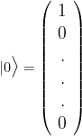
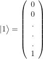
Let us introduce some notation again. Let 

where, 


or

And k=2,
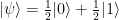
The superposition principle is one of the most confounding and mysterious phenomena of quantum mechanics. You can think of it as the electron not being able to make its mind as to which state it occupies. And α0 is the inclination of the electron to live in the ground state. Here, you might be tempted to call α0 the probability of the electron being in the ground state. But remember that? α is a complex number, so it can be negative or imaginary. It is precisely the amplitude. Don’t worry, we will address it later as we talk about the measurement principle.
The Hilbert Space
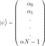
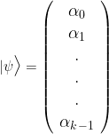
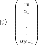
Let’s return to the Bra-ket notation. The quantum state of a k-state is represented by a sequence of complex numbers
Here’s the beauty, the normalization of the vectors means that the state of the system is a unit vector and this allows us to represent the state space in a k dimensional vector space. It looks something like this:
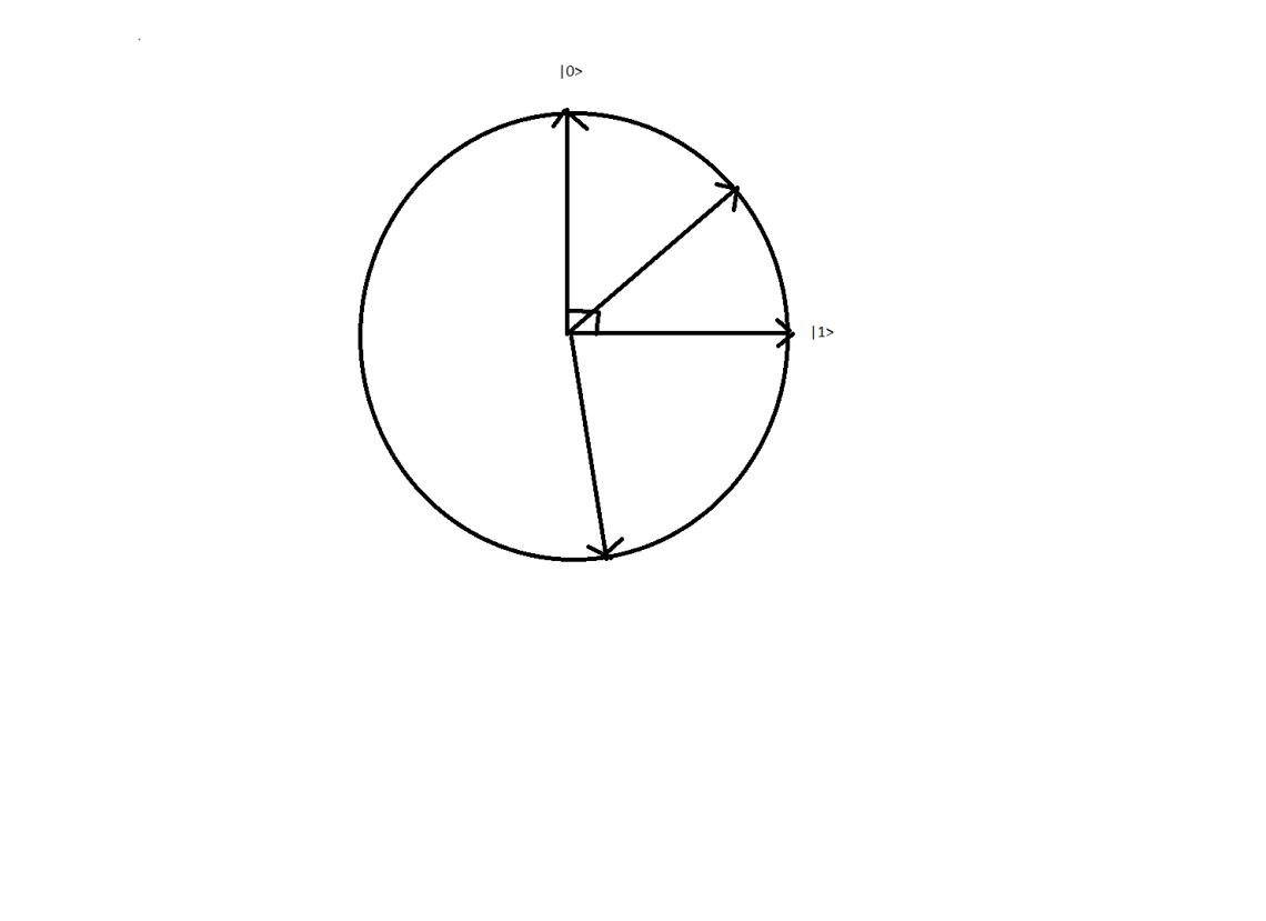
Fig: A representation of quantum states as vectors in a Hilbert Space
Hold your horses though. We are not done yet. If you remember, we wrote the quantum state as 
This notation is called Dirac’s ket notation and is a much simpler and effective way of writing vectors. However, we have a beautiful geometric interpretation of the states in which the vectors can be represented as mutually orthogonal (in right angles to each other) in a k dimensional complex vector space. Or, in other words, they form an orthonormal basis for that space (also called the standard basis).
For any two given vector spaces, 


If you are a bit familiar with quantum mechanics, you can appreciate the convenience of the ket notation. But I will assume you are not. The ket notation allows us to explicitly state the quantum state as a vector while showing the physical quantity of relevance and interest.
I have been talking about the inner product but I haven’t told you what it is. Its roots are in linear algebra. If you are a tad familiar with vectors, you will see that it is linked to the dot product. In very simple words, it is a mechanism to get a number from two vectors.
Let us define 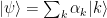
We can calculate the inner product of 
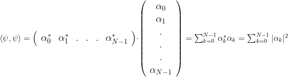
You might wonder why we took the complex conjugate. We did that so that we can obtain a number or a corresponding length. Dirac thought that there must be an easier way out. So, he devised the bra. A bra is defined as the conjugate transpose of a ket and looks like this:

The bra acts on an object to give number as long as we remember that
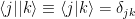
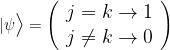
Where, j and k are orthogonal vectors and δjk is called the Kronecker delta, which in turn is defined as:
Now, we can write the inner product of 
The same can be applied for two separate vectors.

If you tinker a little (which I highly recommend doing), you will find that the inner product is not necessarily real and hence belongs to the complex space.
A bra is very much like a function and hence is called a “functional” as when fed with a ket, it returns a number. The space formed by all the bra vectors is called the dual space and it is the set of all the linear functionals that can act on the Hilbert space.
Now, we are all geared up to tackle the measurement principle.
The Measurement Principle
Electrons are fiercely private. And we constantly try to evade that privacy, even though access to information is severely limited. How? We cannot actually measure the complex amplitude αj. And this limitation is encompassed by the Measurement Principle.
A maximum of k outcomes are possible when 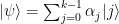


You might try to devise another way to know more about the amplitudes or probe the Hilbert space but measurement is the only way to do so, at least until now. The selection of the basis is important and it is generally done by selecting an orthonormal basis and the outcome of the measurement is 
We will be returning to the detailed technicalities and the physical implications and procedures of the measurement principle later on in a different article (qubits!!!).
Unitary Evolution Principle
The unitary evolution principle on a first glance is peculiar too. It tells us how a quantum state evolves in time. It states that a closed quantum state is described by a unitary transformation. The state 


But what is a unitary operator (the mathematically inclined reader can skip this paragraph)?
A unitary operator is a bounded linear operator 
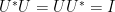


Here, 

Just the way quantum mechanics doesn’t tell us what state the particle is in, it doesn’t tell us which unitary operators describe the dynamics of such a system. It merely assures us that there is a way the system evolves in time. But which unitary transform to choose? Interestingly, in the case of k = 1 (or single qubits), any unitary operator can be realized in realistic systems.
The postulate also requires the quantum system to be closed or it is not interacting with the surroundings in any way. But, apart from the Universe as a whole, nothing is closed (let it sink in for a while and ponder about it, you won’t be disappointed). I can assure you however that there are very interesting systems which are close to closed and which can be described by unitary evolution to a certain degree. With some manipulation we can also describe an open or relatively open system as a part of a larger closed system (guess what it could be) undergoing unitary evolution.
We can also formulate a more refined formalism for evolution of a quantum system in continuous time. However, I will save that for later for it requires some form familiarity with the Schrodinger’s equation and linear algebra.
You might also wonder why the operator has to be unitary. Well, a simple way to put it would be that time evolution should preserve the normalization we have chosen for the initial state because the probability of finding 
We have a reached the end of the preparation for the journey to go about exploring the myriad world of qubits. You now have all the formalisms (probably a bit more) to tackle the basics of the qubit. We would take detours from qubits to explore the world of quantum mechanics in more detail, but till then, this is Baibhav signing off! If you have any doubts or opinions comment away. Don’t forget to leave a like and subscribe!
Further reading:
- The mathematically inclined reader can check out Nielsen and Chuang’s “Quantum Computation and Quantum Information” Cambridge press.
- John Preskill’s introduction to quantum computation is another excellent introduction to the subject.
- MIT’s 8.04 serves as an excellent introduction to quantum mechanics. It has two of my favorite professors, Prof. Adams and Prof. Zwiebach.
- R. Shankar’s Principles of Quantum Mechanics, 2nd Edition, Springer is an excellent text with challenging problems. Apt for the motivated reader.

Very informative article. Keep on writing.
LikeLiked by 1 person
Thank you!!
LikeLike
It’s difficult to find knowledgeable people about this topic, however, you sound like you know what you’re talking about! Thanks
LikeLiked by 1 person
Thanks! Keep following Feynmand! Have a great day! 🙂
LikeLike
always i used to read smaller content which also clear their motive, and that is also happening with this article which I am reading now.
LikeLiked by 1 person
Thank you! 🙂
LikeLike
Hi there! I know this is kinda off topic however I’d figured I’d ask.
Would you be interested in exchanging links or maybe guest writing a blog article or vice-versa?
My site goes over a lot of the same subjects as yours and I
think we could greatly benefit from each other. If you might be
interested feel free to send me an email. I look
forward to hearing from you! Terrific blog by the way!
LikeLike
Wow, great article.Really thank you! Keep writing.
LikeLike